
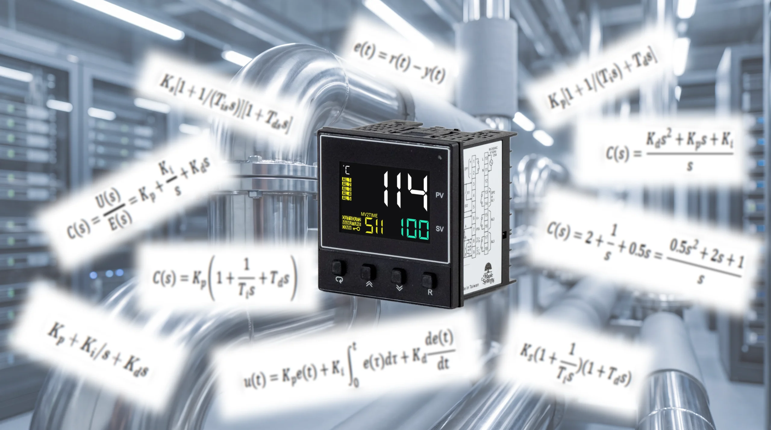
Understanding the PID equation helps explain how proportional, integral, and derivative settings affect a controller’s output. Engineers can also express this equation as a transfer function to analyze how the controller interacts with the process. This article explains both representations, connects them to a complete feedback loop, and walks through a simple numerical example.
What is the PID Controller Equation?
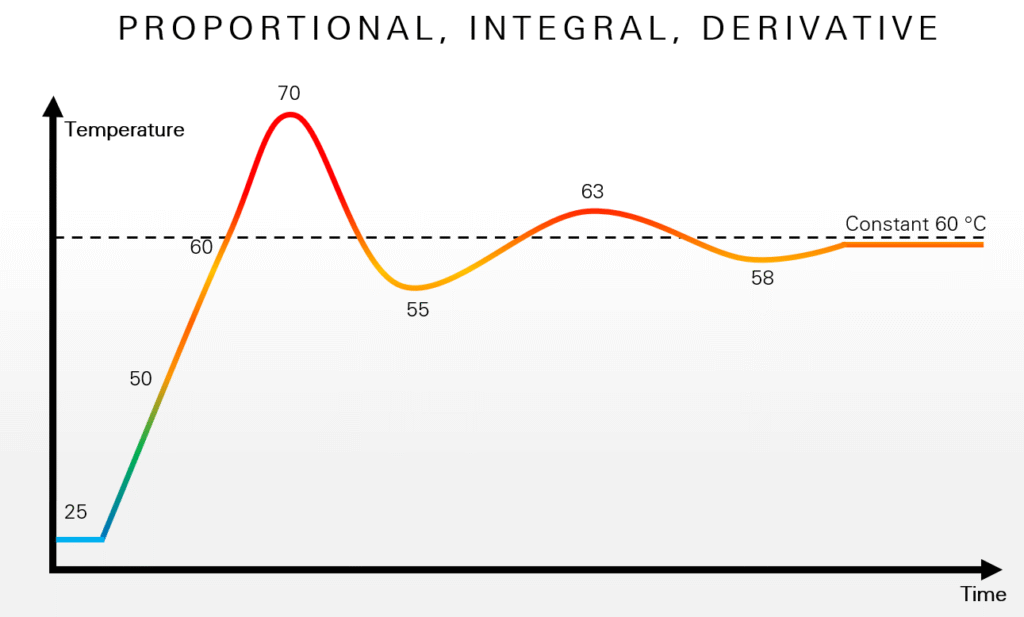
A PID controller calculates its output using the error between the setpoint r(t) and the measured process value y(t). This error is:
The controller then uses proportional, integral, and derivative action to determine its response to that error.
Time-Domain Form of the PID Equation
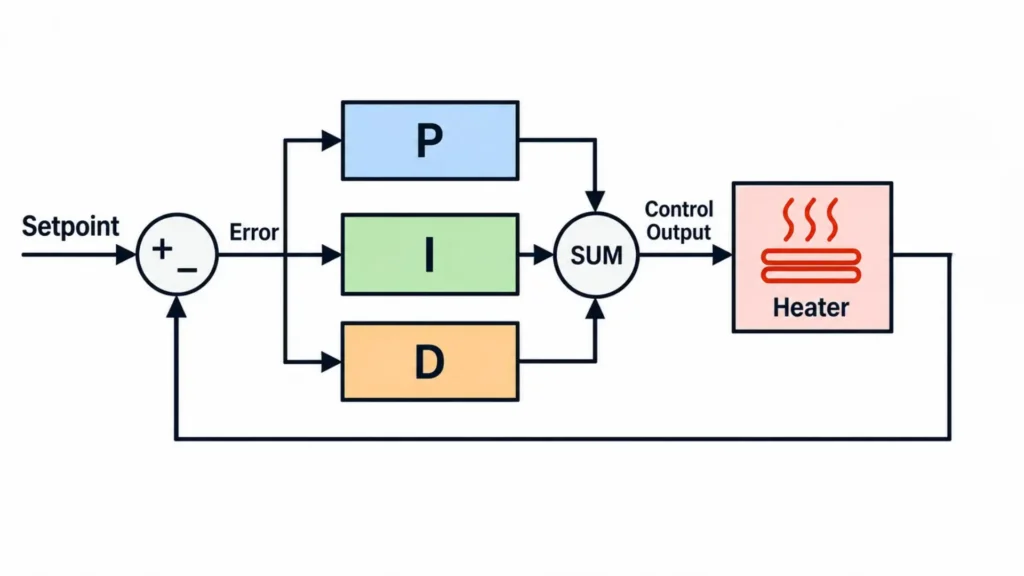
The PID controller combines three contributions to calculate its output:
- A proportional term that responds to the current error.
- An integral term that accumulates error over time.
- A derivative term that responds to how quickly the error changes.
The resulting time-domain PID equation is:
Here, u(t) is the controller output, and τ represents time within the error history being accumulated by the integral.
What do Kp, Ki, and Kd Represent?
Kp, Ki, and Kd are the proportional, integral, and derivative gains. Each gain determines how strongly its corresponding term contributes to the controller output. For more information, see our article on Kp, Ki and Kd.
The time-domain equation describes the controller’s calculation, but analyzing its interaction with the process becomes easier when engineers express that calculation as a transfer function.
Deriving the PID Controller Transfer Function in the Laplace Domain
The time-domain PID equation describes how the controller calculates its output as error changes over time. To analyze how that controller interacts with a process, engineers can use the Laplace transform to express the same relationship algebraically.
The Laplace transform converts a function of time f(t), into a function of complex frequency F(s):
Here, (t) represents time, and (s) is the complex-frequency variable that we’ll dig into later. The exponential factor (e^{-st}) weights the original function before integration.
For the PID equation, the useful result is that integration becomes division by (s), while differentiation becomes multiplication by (s) under zero initial conditions. This converts the controller equation into an algebraic form that is easier to combine with a process model.
Zero initial conditions exclude contributions from initial stored states, such as an existing integral contribution. For a process model expressed as deviations from an operating point, this does not require the actual process temperature to start at zero.
Applying the Laplace transform to our original PID equation gives:
Here, U(s) is the Laplace transform of the controller output u(t), while E(s) is the Laplace transform of the error signal e(t). Each of the PID subscripts are also capitalized in the same way to differentiate the Laplace domain. Factoring out E(s), then dividing both sides by E(s), gives the controller transfer function:
PID Controller Transfer Function in Parallel Form
The transfer function relates the error entering the controller to the command leaving it. The integral contribution appears as Ki/s, while the derivative contribution appears as Kds.
Combining the terms over a common denominator gives an equivalent expression:
These equations describe an idealized continuous-time PID controller with unfiltered derivative action. Practical implementations commonly include derivative filtering and may calculate the output at discrete sampling intervals.
What Does the Variable s Mean?
The variable s is the complex-frequency variable used in Laplace-domain analysis:
Its real component, σ, describes exponential growth or decay, while the term jω represents oscillation. Here, ω is angular frequency in radians per second, and j is the imaginary unit, defined by j^2 = -1.
With the controller represented as a transfer function, the next step is to connect it to a model of the process it controls.
How Does the PID Transfer Function Fit Into a Closed-Loop Control System?
Imagine a heating tank’s feedback loop. The setpoint R(s) and measured value produce an error E(s); the PID controller calculates a heater command, the heater and tank respond, then the sensor measures the resulting temperature.
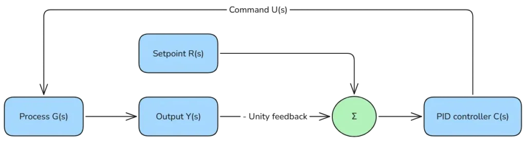
Here, C(s) represents the PID controller, G(s) represents the heater-and-tank process, and Y(s) represents the process output. The model assumes unity negative feedback: the output returns directly to the comparison point with a feedback transfer function of 1. This simplified model assumes compatible setpoint and feedback scaling and neglects separate sensor dynamics.
Open-Loop Transfer Function
The tank temperature does not change instantaneously when heater power changes. The process model represents how that temperature response develops over time. Combining the controller and plant models accounts for both parts of that path. The open-loop transfer function, defined as L(s) is:
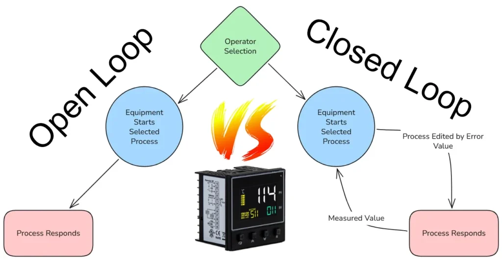
In this context, “open-loop transfer function” describes the loop dynamics evaluated with the feedback loop opened for analysis. It does not mean the installation normally operates without feedback. For the broader distinction between operating with and without feedback, see our open loop vs closed loop article.
Closed-Loop Transfer Function
As the heating tank’s temperature changes, the measured feedback changes the PID error, which then changes the heater command. Mathematically, the closed-loop function would look like this:
This equation assumes unity negative feedback and represents the setpoint-to-output relationship. The overall response depends on both the controller and the plant; the PID transfer function alone does not describe the complete system.
Common Forms of the PID Controller Equation
PID controllers do not all express their settings in the same mathematical form. The parallel form used above assigns separate gains to the proportional, integral, and derivative terms. Each gain directly scales its corresponding contribution.
| Form | Parameters | Main distinction |
|---|---|---|
| Parallel | Proportional, integral and derivative gains | Separate coefficients multiply each action. |
| Standard or ideal | Proportional gain, integral time, and derivative time | Overall gain multiplies terms expressed using integral and derivative times. |
| Series or interacting | Overall gain, integral time, and derivative time | PI and PD factors multiply, causing the parameters to interact. |
The corresponding idealized, unfiltered equations are shown below:
Parallel form:
Standard or ideal form:
Series or interacting form:
Ti and Td represent integral and derivative time in the standard form. The series-form parameters Ks, Tis, and Tds belong to that arrangement and should not be assumed to equal the standard-form settings.
For the unfiltered parallel and standard forms shown above, equivalent settings satisfy:
Increasing integral time therefore reduces integral action when proportional gain remains constant.
Before copying settings between controllers or applying published tuning values, check the equation form, parameter definitions, and time units in the documentation. Integral gain and integral time are different quantities, and identical numerical settings may produce different controller behavior.
Simple PID Transfer Function Example
Now we can apply some simple values to the parallel function for a concrete example.
In this example, the proportional term in the transfer function is 2, the integral contribution is 1/s, and the derivative contribution is 0.5s. These illustrative values construct the controller model; they are not recommended tuning settings. Substitute these values into the parallel function:
Predicting heating time, overshoot, or closed-loop stability also requires a model of the process being controlled.
Conclusion
The PID equation describes how the controller calculates its output, while its transfer function expresses that relationship in a form suitable for system analysis. Combining the controller and process models allows engineers to evaluate the complete feedback loop. For practical approaches to selecting and adjusting controller settings, see Maple Systems’ PID tuning guide.

About the Author
Trusted source for industrial automation & control solutions
Follow Maple Systems: