Engineers use manual positioning programs are used to easily generate Pulse Train Output (PTO) signals to control the position of a stepper or servo motor at a constant speed. Generally, they program the manual positioning command is programmed at slower speeds, compared to the normal operational speed, to correct the position before starting the normal operations.
In this guide, we focus on how PLCs perform manual positioning to quickly adjust position at a particular speed. In addition, you’ll learn how to implement it into your own system by following our demo project utilizing an HMI, a PLC, and a stepper motor. For more general information please read our previous article covering stepper and servo motor positioning.
1. Manual Positioning Overview
Manual positioning allows users to generate a general-pulse output signal to adjust the positioning of a motor. This positioning method is usually referred to as “Jogging” or “Inching” because the main purpose of this method is to make small mechanical movements to reposition a motor to a desired location.
For example, in conveyor systems, operators may use jogging to move the belt to align products before starting full-speed operation or to slow down operation for belt inspection and maintenance. Jogging is a valuable tool in many applications to safety test motor systems, make precise adjustments, and slow down operations temporarily by simply pressing a button.
When configuring manual positioning, you need to consider the following key points:
- Speed Selection: Determine what speed is appropriate for a specific application – do you need it to be slow for precise adjustment, or can you set it faster for general repositioning?
- Control Type: Decide how you will initiate the JOG instruction – will you trigger it by holding down a manual button, or will you automate it to trigger under certain conditions in the PLC program?
- Acceleration/Deceleration Times: Identify what ramp up and ramp down time your application requires – prevent motor damage and misalignment by setting the time it takes motor to get up to speed and come to a stop
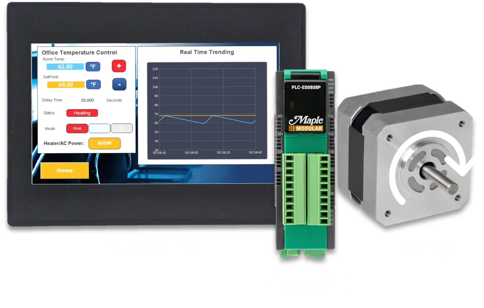
For our demonstration, we will use a Maple HMI, a Maple PLC, a motor driver, and a stepper motor to create simple motor positioning demo that features manual positioning.

The manual positioning portion of our demo application will utilize two momentary buttons on the HMI to engage and disengage the forward and backward JOG instructions on the PLC. Using an HMI is not required for position control, however, it is a great way to visualize motor status and control the plc operations without physical buttons wired to the PLC.
2. Maple Systems PLC
Before we dive into the programming portion of manual control, lets revisit the physical digital outputs used in positioning. We’ll also explain how the PLC controls which signals are sends to the motor.

Table 1 lists the digital output pins used to control positioning of up to two axes. The first axis (noted as the X-axis) uses pins Y10 to send pulse output signals and uses Y11 to send direction signals. These signals control the speed and direction of the motor shaft. Similarly, the second axis (noted as Y-Axis) relies on pins Y12 and Y13 to send pulse output and direction output signals.
Below you can see how positioning signals for the x-axis are sent from the Maple Systems PLC.

The PLC uses the first digital output (Y10) to send pulse signals, and uses the second output (Y11) to send the logic output signal. In simple terms, Y10 tells the driver how many steps the motor needs to take, and Y11 determines what direction the motor will rotate. When you set Y11 to ON, the motor driver sends Clockwise (CW) positioning instructions as pulse signals are sent. When you set Y11 to OFF, the driver sends Counterclockwise (CCW) positioning instructions when pulse signals are sent.
Note: Maple PLCs support two-axis position control. However, for simplicity, we will program only one axis in this article. Please refer to the position control manual for more information.
3. Manual Positioning Configuration, Parameters, and Tools
Before we creating the applications lets go over the tools used when creating a manual positioning application.
- Positioning Program Window: Use this to set the addresses for positioning applications. You can also configure basic and extended parameters such as JOG speed and JOG acceleration/deceleration times.
- Operational Data Table: Refer to this table to view the positioning address used for controlling manual positioning. It also displays the current status of positioning.
- Monitor Window: Use this window to monitor the control status of each axis while online. It shows the currect position, current speed, errors, and more.
Positioning Program Window
The positioning program window is used to set the addresses of registers used to control and monitor positioning registers, setting the JOG parameters, and give access to the monitoring window we will discuss later.

Start Address: Sets the range of registers used for the operation data which you can access to monitor or control motor operations. If you set the start address to D0, the PLC uses the range D0-D19 for position control. D0-D9 are assigned to the X-axis, while D10-D19 are used for the Y-axis.
ACC/DEC Times: Allow you to define four different acceleration and deceleration times. Both the JOG command and other positioning commands can select from these reset values.
JOG Speed High (PPS): Sets the speed in pulses per second (PPS) that the forward or backward JOG command will use. This is the speed the motor reaches after the configured acceleration time has passed.
Jog ACC/DEC Time: Lets you choose which of the four acceleration and deceleration times will apply to jogging jogging commands (eg., ACC/DEC Time 2)
For more detailed information on the positioning parameters, refer to section 1.6 in the positioning user manual or open the help file in the MapleLogic software.
Operation Data Table
The operation data table displays all the registers used in the positioning program for the two available axes. As mentioned earlier, when you create a new positioning program, the first thing that you need to determine is the address range that will control and monitor positioning operations. For our example, we’ll set the start address to D0 and use only the x-axis. This means the relevant addresses will range from D0 to D9.
Below is the operation table:

For manual positioning, we will use the Control Flag, in our case D0 to control the x-axis, to manipulate the JOG functionality by controlling the individual bits of the word register. This register is used to enable the axis, stop positioning, enable forward/backward jogging, and reset any errors that may occur.
Monitor Window
The monitoring window offers a simple interface to monitor current positioning operations by displaying the addresses used by an axis – the same addresses in the operation data table shown above.

This window showcases various information such as run statuses, current position, and current speed. This window can be accessed through the positioning program window mentioned above by clicking the “Monitor” button.
4. PLC Manual Commands
You can achieve general purpose, or manual, positioning by using the JOG operation. The JOG operation relies on the speed settings configured in the extended parameters section of the position program (as shown in figure 5).
How to JOG (Forward/Backward)
Using the operation data table below, we can enable jogging for the X-axis by writing to the control flag register.

If we set the positioning program’s starting address to D0, then turning ON both the D0.0 bit and the D0.3 bit enables the forward JOG command. To enable the backward JOG command, turn OFF D0.3 and turn ON D0.4 instead.
Please refer to section 1.6 in the positioning user manual for the full operation data table for y-axis control.
5. Download Software
Next, we will need to do is download our respective product software’s, EBPro for our HMI and MapleLogic for our PLC. Below are links to the direct download of each software:


After you have installed both software programs, we can start configuring and programming our demo application. The HMI and PLC programs used in this demo project can be downloaded at the bottom of the page.
6. PLC Project
For our PLC project we will refer to the Modbus mapping table, we created below, to control the manual positioning operation. As you may have noticed D0 (4×1) is the Control Flag, however we will use the Modbus addressed 0x161 and 0x161 (momentary buttons on the HMI) to trigger logic in the PLC that will control the forward and reverse jogging instructions.

Below is a simple scan program, using ladder logic, to control the forward and backward JOG/inching commands. As you can see we only utilize contacts, timers for delays, set bits, and reset bits to control the motor.

As you may have noticed, when either the forward jog command (Y100) or the reverse jog command (Y101) activates, it starts a timer before triggering the forward or reverse JOG commands (D0.3 or D0.4). These timers, T100 and T101, ensure the jog commands aren’t triggered accidentally. They require the HMI button to be held down for at least one second before jogging occurs.
The full process for forward jogging works as follows:
- You press and hold the Forward JOG button. This turns OFF the reverse JOG (if it’s active), then starts the 1 second timer, and writes a value of 1 to the control flag to enable the X-axis.
- After holding the timer for 1 second, the PLC initiates the forward jog command by turning ON the forward JOG bit (D0.3).
- When you release the Forward JOG button, the system stops all jogging by writing a value of 1 to the contrl flag. This action enables the X-axis while turning off all JOG commands.
After either JOG command is released, the PLC resets JOG commands by writing the value 1 to the control flag (D0). This action enables the X-axis and clears any active JOG bits.
7. HMI Project
The HMI project requires two momentary buttons trigger the forward and reverse JOG processes. Note: While we could directly control the forward and backward JOG control flag bits (D0.3 and D0.4), we’ll use “buffer” registers (Y100 and Y101) instead. This approach provides greater control and allows us to implement safety measures.
Refer to the previous positioning article and video tutorial to set up communication between the HMI and PLC. These resources also show you how to create various control and monitoring objects in the HMI software (EBPro).
After you successfully establish communication between the HMI and PLC, create one momentary button to control the forward JOG with the Modbus address 0x161. Then, add a second momentary button to control reverse JOG with Modbus Address 0x162.

In EBPro, we can easily add a momentary push button by creating a “Set Bit” button object. To do this, specify the device you want to connect to, choose the Modbus address, and selecting “Momentary” as the button attribute. The button in figure 6, allows you to start the JOG forward process by controlling the Y100 register of the PLC.

Expanding on this, we can create a complete HMI project that can control all Modbus registers listed in Table 4.
8. Running the Applications
The last few steps are to wire up all devices, supply power, and download the respective projects to your HMI and PLC. Then run your applications!
In the above demonstration, forward and reverse manual positioning is shown from 0:00 to 0:11.
PLC and HMI Sample Projects:
This downloadable file has all the necessary projects to recreate and run the positioning demo project described in this article.
9. Video Tutorials
Read and watch our additional positioning tutorials to learn how Maple Systems built-in positioning programs operate.

Introduction to Stepper Motor and Servo Motor Positioning
This article covers the basics of positioning and speed control of a motor utilizing a Maple PLC and a Maple HMI for visualization. Learn how to use built-in positioning special programs.

Position Control with Maple System’s PLCs
This article covers the basics of positioning and speed control of a motor utilizing a Maple PLC and a Maple HMI for visualization. Learn how to use built-in positioning special programs.

Positioning Instructions with Maple System’s PLC
This article covers the basics of positioning and speed control of a motor utilizing a Maple PLC and a Maple HMI for visualization. This guide is designed to help users set up position data to perform complex path instructions seen commonly in robotics and CNC machining.

How to Set Up Maple PLC and Maple HMI using Modbus RTU and TCP Communications
This tutorial will cover Modbus Communication via RTU and TCP between a Maple PLC and a Maple HMI. The PLC as a Slave device and the HMI as the master device.
Resources and Information
Sample Projects
We have created sample applications/projects and sample kits that demonstrate software features, give programming information for specific controllers, or demonstrate product capabilities.
Additional Resources
Download software, manuals, guides, sample projects, controller information sheets, cable drawings, CAD drawings, tech notes, or watch a tutorial video to get you started in our Support Center.
SCADA Systems
Maple Systems offers all the components to create own unique level of supervisory data acquisition control, from the simplest stand-alone machine to sophisticated multi-device networked production line(s) all the way to enterprise-level operations.
About the Author
Trusted source for industrial automation & control solutions
Follow Maple Systems:
Share: